Pupillometry Walkthrough
This page aims to provide you with a brief introduction to the methods of pupillometry as used in psychology and cognitive science. This is by no means an extensive introduction. For that, you should consult the references at the bottom of the page. Rather, this page presents a simple task, for which data were obtained, and the steps through which these data can be made to tell us anything!
I will provide the data and scripts to reproduce the analyses performed here. At the moment, these are only available for Matlab. If you are the kind of person who would take these and save them in a different format (e.g., R), there may be others who would like to use an alternative to Matlab, so please feel free to send me your alternate files!
Method
Participants
Nine students and staff affiliated with Laboratoire CogNAC from UQTR took part in the study. They were 6 women and 3 men, aged between 21 and 42. They took part in this experiment as part of a workshop on pupillometry. Equipment failure rendered data from one woman participant unusable.
Stimuli and apparatus
A simple arithmetic task was used. Participants were shown 6 addition problems, shown in Figure 1. Half of these problems did not require digits being carried over in order to solve the problems and were labeled easy. The other half of problems required a carry operation in all columns and were labeled hard.
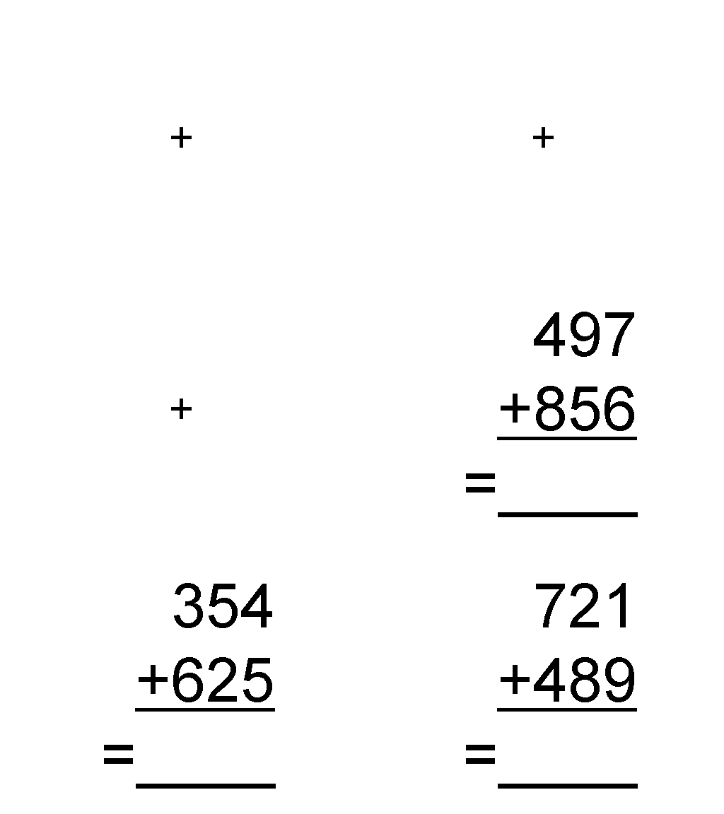
Figure 1. Animation of the 6 problems used in the experiment. This is an endless loop, so please stop after you have seen six problems!
Data were recorded using a Tobii T120 eye tracker, pictured in Figure 2. Sampling rate for this experiment was set at 60Hz.
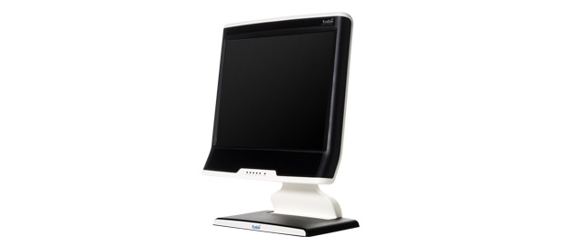
Figure 2. Eye tracker such as used in this experiment.
Procedure
Participants took part, one at a time, in a quiet testing cubicle. They were told they would have to perform six sums outloud, and that each problem would be displayed for 10 seconds. The experimenter sat behind participants, reminding them to solve the problem outloud if they failed to do so. The eye tracker was calibrated using a 5-point procedure.
Each participant saw the same sequence of problems, alternating easy and hard problems. These were presented with the E-Prime 2.0 software package, using Tobii extensions for E-Prime. A fixation cross was shown in the middle of the screen at the start of each trial. When participant had looked at the fixation for at least 100ms, the fixation was replaced by one of the six problems.
Results
Before pupil data can be analysed, a degree of pre-processing needs to take place. Using E-Prime with the extensions for Tobii, we export eye tracking samples to a tab-delimited text file that contains many variables, some relating to time stamps, some relating to gaze, two relating to pupil diameter (one estimate per eye, per sample), and some relating to study variables, such as trial number, on screen stimulus, etc. We have developed some Matlab scripts to help with data extraction, but these are idiosyncratic to how we use E-prime to export eye tracking data, and would not immediately work for some other software/hardware combinations. However, here is the raw data for the relevant variables, in a format that, we feel, is helpful for processing and analyses:
If you load this file in Matlab, you will end up with a structure called data, with 8 fields where each field is a structure relating to the data for each participant. The command data(6) at Matlab's command prompt will see Matlab tell you what information is stored for participant 6. Of that information is the trial_data structure, which contains the data for each of the six trials the participant completed. The command data(6).trial_data(1) will further tell you what data is available for participant 6 on his or her 1st trial. In this case, we have a field called trial_ID (with value 'Easy1'), a field called subset (unused in this study and set to 'none'), two fields (CursorX and CursorY) with gaze coordinates on x and y respectively for all 819 samples of the trial (stored as column vectors), and two fields (LPupil and RPupil) with estimates of pupil diameter for left and right eyes respectively for all 819 samples (stored as row vectors).
The keen and observant reader may wonder why participant 6 provided 819 samples of data on trial 1. The method suggests a trial length of 10 seconds and a sampling rate of 60Hz, leading to an expected 600 samples. This is because of the way we have recorded (and extracted) the data, whereby each trial contains as well the initial portion when the fixation cross was displayed. Participants had to fixate that cross for 100ms (or 6 samples) before the problem was shown. But how long after fixation cross onset they made that critical fixation varied between trials and between participants. Participant 6 has 219 extra samples (or 3.65 seconds) of data on trial 1. We can assume he or she successfully fixated on the cross 3.55s after it was displayed. While we could figure out the exact onset of problems for each participant on each trial, we know that the problems per se were shown for 10 seconds, and therefore we can merely select the last 600 samples of each trial for analyses.
With this in mind, we will first look at the raw data in order to illustrate two important features of pupillometry. Figure 3 shows the raw data from all 8 participants on the last (hard) problem. You can reproduce this figure by running the script found here (2Kb). What the figure shows is that participants have different pupil diameters, and in this case there appear to be two subsets of participants clustered around 2.75 and 3.75mm respectively. This can obviously introduce noise in analyses, and reduce effect sizes. The other important feature is that there are gaps in the data. These are due to eye blinks, or from participants moving their heads in such a way that the eye tracker momentarily loses the ability to track. These are the two main problems we address in pre-processing of data.
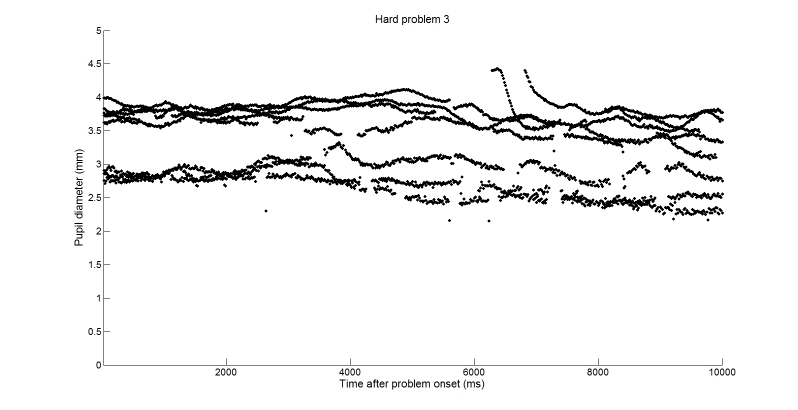
Figure 3. Raw data from all participants on the last trial.
To deal with missing samples, we have developed a method where pupil estimates from each eye are regressed onto estimates from the other eye, and linear interpolation is used to fill in gaps (Jackson & Sirois, 2009). In order to minimise errors due to excessive sampling error at the onset or offset of gaps, data are smoothed using a low-pass filter before interpolation. This procedure allows us to have usable samples throughout trials, and is a simple and elegant solution that is unrelated to any specific research question that pupillometry is used for. Figure 4 illustrates the outcome of this procedure on the same trial shown for raw data in Figure 3.
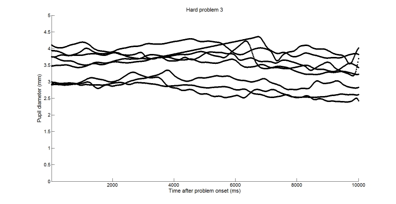
Figure 4. Cleaned data from all participants on the last trial.
You can reproduce Figure 4 by running the script found here (2Kb), using the Clean data object (986Kb). We will use that script and dataset for the rest of the walkthrough, as we will keep working with the cleaned up data. The script uses Matlab's cell mode, meaning that the whole script is broken into chunks using the %% characters. Figure 4 was created in the first chunk of the script. The next chunk deals with baseline removal.
As figures 3 and 4 show, participants differ in their baseline pupil diameter. We do seem to have two distinct subsets in this sample. This wouldn't matter with repeated-measures analyses (such as we will use), which naturally control for such variability. But these analyses are not adversely affected by baseline removal, whereas other analyses as well as descriptive statistics (such as the mean) will benefit from baseline removal. Arbitrarily, we will use the last 3 samples (or 50ms) before the onset of each problem, and subtract the mean of these from all the samples collected while the problem was displayed. This means that we will look at the change in pupil diameter during problem solving, rather than absolute pupil diameter. The script will perform this baseline removal, and produce what is shown in Figure 5.
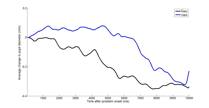
Figure 5. Average change in pupil diameter as a function of problem type.
The data in Figure 5 are quite interesting. As expected, pupil diameter is larger and for longer when participants attempt to solve hard problems, relative to easy ones. But as much as it may be obvious from looking at the figure, the question now is how do we analyse the data to show whether this is a significant difference or not. Commonly, researchers use key time points from which they compute mean change for different conditions, and use traditional statistical procedures (t tests, ANOVA...) on the discrete values they have extracted from the samples. A problem with such approaches is that the size and position of the temporal window within which to extract data is going to be largely arbitrary. And if findings are significant, how robust are they to changes in those arbitrary parameters (e.g., sample 50ms earlier for 100ms longer)? Regardless, this is a common approach and we will illustrate here.
We chose 5 different times at which to compare the performance of participants between easy and hard problems: 0, 2, 4, 6, and 8 seconds from problem onset. We took the mean of each participant for each problem type, and then the median pupil diameter within 100ms after these key times. The results are shown in Figure 6. The Matlab script produces an array named ANOVA_data, the contents of which can be copied into the statistical package of your choice (e.g., SPSS). We performed a 5 by 2 repeated-measures ANOVA with time and problem type as factors, and pupil diameter as the dependent variable. The analysis shows a significant interaction between time and problem type (F(4,4) = 4.418, p = 0.007), as well as significant main effects for both time (F(4,4) = 15.715, p = 0.00) and problem type (F(4,4) = 9.768, p = 0.017). Polynomial decomposition of the interaction reports significant linear, cubic, and quartic relationships. The effect of time is both linear and quadratic. These results are consistent with our eyeballing of Figure 5. Mental effort or load, indexed by pupil diameter, decreases more quickly and steadily on easy problems, relative to hard ones.
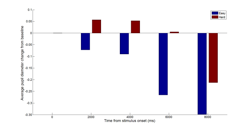
Figure 6. Average change in pupil diameter as a function of problem type at key times during trials.
While the result of the above analysis is great (we have a significant effect!), it relies on methods where we have reduced rich data (8 participants x 6 trials x 600 samples = 28800 data points) to a handful of data (8 participants x 2 problem types x 5 key times = 80 data points). This degree of reduction seems unfortunate, and relies on arbitrary decisions that could miss important effects in the data (or, just as bad, focus on and enhance other effects). This is why we have focused on a different approached based on Functional Data Analysis (FDA: Ramsey & Silverman, 1997). With this approach, we transform data into smooth curves (b-splines), and perform the analyses on those curves. The beauty of this approach is that our statistics are not mere discrete numbers (e.g., F(4,4) = 4.418), but curves too. Therefore, we can look at our F ratio or t test over time, and observe (without arbitrariness) if and when it suggests a significant difference between conditions, a significant interaction, etc.
In order to use the FDA section of the script, you will need to install the set of functions made available by Jim Ramsey on the FDA web page. If all goes well, you are going to be able to reproduce Figure 7 below. This is the average difference between hard and easy problems, computed from b-splines created for each participant.
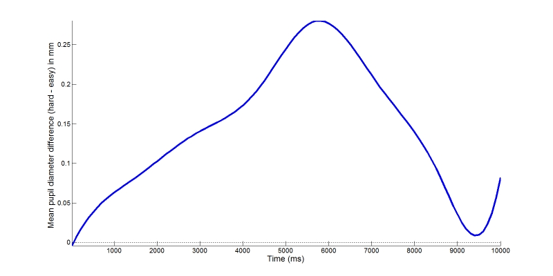
Figure 7. Mean functional pupil diameter difference between easy and hard problems.
We can perform a single-sample t test on this functional data, comparing the average difference to 0, the lack of difference. The result is shown in Figure 8. Hard problems lead to significantly larger pupil diameter, briefly at the onset of trials, and in a more sustained fashion throughout the second part of the trial..
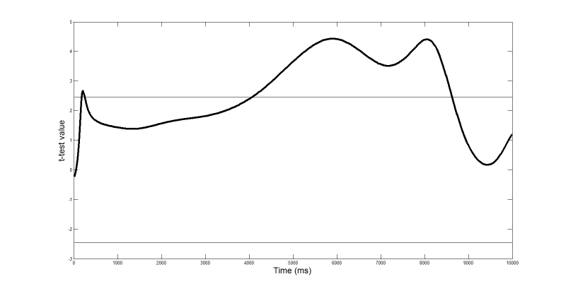
Figure 8. Functional t test of the difference between easy and hard problems. Horizontal lines represent the critical value of the relevant (df = 7) t distribution.
Conclusions
This page has shown the relative ease of carrying out pupillometry research within psychology and cognitive science. We had a simple study, where people had to perform mental arithmetic. The two types of problems, easy and hard, made for a simple prediction: if pupil diameter is an index of mental effort, the pupils should be relatively larger, for relatively longer, on hard problems. The results, derived from a very small sample, highlight both the usefulness and robustness of pupillometry. Pupil diameter changes over time. In relation to cognitive processes, the rate and duration of this change is informative about underlying mechanisms. This is why we have been keen to use statistical methods that not only preserve the richness of temporal data, but that actually capitalize on it. In the process, we have shown that we can analyze how pupil diameter changes over time, as a function of stimulation, removing the need for arbitrary decisions about when and for how long to look for effects based on a discrete summary of that rich data. As an analogy, if you think of pupil diameter as an honest witness of mental activity, traditional methods that average pupil data at fixed times are like asking "where were you at exactly 150ms?". Approaches such as the FDA one we favor are a different kind of interrogation technique, like asking "can you tell us everything that happened after the stimulus entered the room?". We think the latter interrogators, if they have the right statistical tools, will make a much stronger case about what actually happened. Personally, we think the hippocampus did it.
References
Brisson, J., Mainville, M., Mailloux, D., Beaulieu, C., Serres, J., & Sirois, S. (2013). Pupil diameter measurement errors as a function of gaze direction in corneal reflection eyetrackers. Behavior Research Methods, 45(4), 1322-1331.
A paper on how some eye trackers make systematic errors in pupil diameter estimation, and how to fix them. Link
Fitzgerald, H. E., Lintz, L. M., Brackbill, Y., & Adams, G. (1967). Time perception and conditioning an autonomic response in human infants. Perceptual Motor Skills, 24(2), 479-486.
The original paper on pupillometry with infants. Link
Hess, E. H., & Polt, J. M. (1960). Pupil Size as Related to Interest Value of Visual Stimuli. Science, 132(3423), 349-350.
The seminal paper for contemporary pupillometry in psychology. Link
Jackson, I., & Sirois, S. (2009). Infant cognition: going full factorial with pupil dilation. Developmental Science, 12(4), 670-679.
Our paper introducing FDA in pupillometry. Link
Laeng, B., Sirois, S., & Gredeback, G. (2012). Pupillometry: A Window to the Preconscious? Perspectives on Psychological Science, 7(1), 18-27.
A review of pupillometry in psychological sciences. Link
Ramsay, J. O. and Silverman, B. W. (1997). Functional Data Analysis. New York: Springer-Verlag.
Original book on FDA. The website has many resources. Link
Learn more!
Contact me by email: sylvain.sirois@uqtr.ca